Understanding Support Vector Machine (SVM) Algorithms

Introduction:

Machine learning algorithms strive to make sense of complex data and unearth patterns. One particular method has risen to prominence for its efficacy in classification tasks—Support Vector Machine (SVM) Algorithms. As we navigate the intricacies of machine learning, it becomes imperative to comprehend the inner workings of SVM algorithms. And we need to appreciate their role in shaping intelligent systems.

Machine learning is about empowering computers to learn from data and make decisions or predictions. In this pursuit, classification algorithms play a pivotal role, enabling machines to categorize information into distinct groups. SVM stands tall among these algorithms. It has garnered attention for its ability to find optimal decision boundaries. That makes it a linchpin in various applications, from image recognition to financial forecasting.

In this exploration, we embark on a journey to demystify Support Vector Machines. We will unravel the fundamental concepts that underpin SVM, from the notion of hyperplanes to the significance of support vectors and margins. Along the way, we will delve into the diverse landscape of SVM kernels. Each one is serving as a tool in the hands of data scientists to navigate different data scenarios.

Understanding SVM is not just an exercise in comprehending a machine learning algorithm; it’s an invitation to harness the power of intelligent classification. It is gaining insights into its advantages. It acknowledges its limitations. And it is ultimately discerning when and how to deploy it effectively.

So, let us venture into Support Vector Machines. And decode the complexities that lie beneath the surface. And shed light on the brilliance that makes SVM a cornerstone in the ever-evolving world of machine learning.

Introduction to Machine Learning and the Significance of Classification Algorithms:

In technology, data has become the currency of insight. Machine learning emerges as the driving force behind intelligent decision-making. Machine learning is a branch of artificial intelligence. That empowers computers to learn from experience. And it automatically improves their performance without being explicitly programmed. At its core, machine learning seeks patterns within data. And it is transforming raw information into actionable knowledge.

Classification holds a paramount position within the expansive toolbox of machine learning algorithms. Classification algorithms are the engines behind systems that organize and categorize data into predefined classes or labels. This categorization forms the backbone of various applications, from email spam filters to voice recognition software. It enables machines to make informed decisions by associating input data with predefined outputs.

The importance of classification algorithms lies in their ability to generalize from known examples and apply this knowledge to new, unseen data. In a world inundated with information, the capacity to automatically classify and organize data not only streamlines processes. It also opens doors to innovative solutions across diverse domains.

Let us embark on our exploration of Support Vector Machines (SVM). Further, let us understand the broader context of machine learning. In addition, let us learn the pivotal role of classification algorithms, which sets the stage for comprehending the nuanced brilliance of SVM in handling complex classification tasks. So, let us unravel the intricacies of these algorithms and appreciate their significance in the ever-evolving landscape of intelligent computing.

The Pivotal Role of Support Vector Machine (SVM) Algorithms in Machine Learning:

Within the vast repertoire of machine learning algorithms, Support Vector Machines (SVMs) stand out as powerful tools for tackling complex classification problems. The distinctive strength of SVMs lies in their ability to discern optimal decision boundaries in data. That makes them invaluable in scenarios where precision and accuracy are paramount.

SVM is a supervised learning algorithm that excels in both linear and non-linear classification tasks. Traditional algorithms merely categorize data points. At the same time, SVM goes a step further and identifies the optimal hyperplane. An optimal Hyperplane is a decision boundary that maximizes the margin between different classes. This enhances the algorithm’s ability to generalize to unseen data. And it further fortifies its resilience in the face of noise and outliers.

The key concept driving SVM’s efficacy is the notion of support vectors—data points that exert the most influence in defining the decision boundary. By strategically selecting these support vectors, SVM creates a robust model less susceptible to Overfitting and generalizes well to diverse datasets.

SVMs have proven instrumental in a myriad of applications. It is more efficient in image, speech recognition, financial forecasting, and bioinformatics. Their versatility extends to scenarios where the relationships between features are intricate and the data is not easily separable. Through the adept use of kernel functions, SVMs can efficiently handle non-linear mappings. That is further expanding their applicability.

Support Vector Machines embody the essence of intelligent decision-making in machine learning. Their capacity is to discern nuanced patterns, coupled with a robust mathematical foundation. That makes them indispensable in the pursuit of building accurate and adaptable models. As we delve deeper into the intricacies of SVMs, we uncover a tool that not only classifies data. But it also elevates the standards of precision and reliability in the ever-evolving landscape of machine learning.

Support Vector Machine (SVM) Algorithms: A Fundamental Overview

Support Vector Machines (SVMs) are a class of supervised machine learning algorithms designed for classification and regression tasks. It was developed by Vladimir Vapnik and his colleagues in the 1960s and 1970s. SVMs have become a cornerstone in machine learning due to their robust performance in high-dimensional spaces and adaptability to various data types.

At its core, SVM is a binary classification algorithm. It categorizes data points into one of two classes. The fundamental principle guiding SVM is the identification of an optimal hyperplane in the feature space that best separates the different classes. This hyperplane is strategically positioned to maximize the margin—the distance between the hyperplane and each class’s nearest data points (support vectors). By maximizing the margin, SVM aims to enhance the algorithm’s generalization ability to new, unseen data.

Key components of SVM:

1. Hyperplane: The decision boundary that separates different classes. In a two-dimensional space, it is a line. In higher dimensions, it becomes a hyperplane.
2. Support Vectors: Data points that influence the most on determining the optimal hyperplane. These are the points closest to the decision boundary.
3. Margin: The distance between the hyperplane and the nearest support vectors of each class. Maximizing the margin is a critical objective in SVM.

To handle non-linearly separable data, SVM employs kernel functions. That allows it to implicitly map data into higher-dimensional spaces where a linear separation becomes possible.

SVMs find applications in various domains, including image and text classification, bioinformatics, finance, etc. It handles both linear and non-linear relationships coupled with robust generalization properties. This ability makes SVMs a versatile and powerful tool in the machine learning toolbox. As we delve deeper into the intricacies of SVMs, we uncover this sophisticated algorithm that continues to contribute significantly to the advancement of intelligent systems.

Support Vector Machine (SVM) Algorithms: Definition and Significance in Classification Tasks

Definition:

Support Vector Machines (SVMs) are a class of supervised machine learning algorithms used for both classification and regression tasks. SVMs are particularly adept at binary classification. In this case, the algorithm assigns input data points to one of two classes. The fundamental principle behind SVM is to find the optimal hyperplane in the feature space that best separates different classes. It maximizes the margin between them.

Significance in Classification Tasks:

1. Optimal Decision Boundary:

   SVMs excel at identifying the most effective decision boundary (hyperplane) between classes. This optimal decision boundary maximizes the margin. The optimal decision boundary is the distance between the hyperplane and the nearest data points of each class. The larger the margin, the better the SVM generalizes to new and unseen data. It reduces the risk of misclassification.

2. Handling High-Dimensional Data:

   SVMs perform well in high-dimensional spaces. That makes them suitable for scenarios where the number of features is significant. This is crucial in modern datasets where numerous variables often represent information.

3. Robustness to Outliers:

   The choice of the optimal hyperplane in SVM is influenced by support vectors—data points that are closest to the decision boundary. This approach makes SVM robust to outliers since the impact of outliers is mitigated by focusing on the critical support vectors.

4. Versatility with Kernels:

   SVMs can handle both linearly and non-linearly separable data through the use of kernel functions. These functions implicitly map data into higher-dimensional spaces. It makes complex relationships discernible and expands the applicability of SVMs to a wide range of problems.

5. Generalization to Unseen Data:

   SVMs aim to find decision boundaries that generalize well to new data. This characteristic is vital for creating models that are accurate on training data and perform well on real-world instances.

6. Applications Across Domains:

   SVMs find applications in diverse fields, such as image and speech recognition, text categorization, bioinformatics, finance, and more. Their versatility and effectiveness make them a popular choice in various real-world scenarios.

In summary, Support Vector Machines play a pivotal role in classification tasks by efficiently finding optimal decision boundaries. It handles high-dimensional data and offers robustness and versatility through the use of kernels. Their significance extends to a wide array of applications. That makes them a key player in the realm of supervised machine learning.

Basic Idea of SVMs In Terms Of Finding the Optimal Hyperplane for Classification

The basic idea behind Support Vector Machines (SVMs) lies in finding the optimal hyperplane for classification. The optimal hyperplane is crucial in SVM as it serves as the decision boundary that maximizes the margin between different classes. Here is a step-by-step explanation:

1. Data Representation:

   • Consider a dataset with input features, each associated with a class label (either +1 or -1 for binary classification). In a two-dimensional space, the data points can be plotted. Each point is represented by its feature values.

2. Linear Separation:

   • SVM aims to find a hyperplane that effectively separates the data into different classes. In a two-dimensional space, this hyperplane is a line. In higher dimensions, it becomes a hyperplane.

3. Maximizing Margin:

   • The margin is the distance between each class’s hyperplane and the nearest data points (support vectors). The goal is to maximize this margin. Intuitively, a larger margin suggests a more robust decision boundary that generalizes well to new, unseen data.

4. Identifying Support Vectors:

   • Support vectors are the data points that lie closest to the decision boundary. They play a pivotal role in defining the optimal hyperplane. The optimal hyperplane is positioned to be equidistant from the nearest support vectors of each class.

5. Mathematical Formulation:

   • Mathematically, the optimal hyperplane is defined by an equation that expresses a linear relationship between the input features. In a two-dimensional space (for simplicity), the equation of the hyperplane is given by w⋅x+b=0w⋅x+b=0. Where ww represents the weights assigned to each feature. xx is the input feature vector. And bb is the bias term.

6. Optimization Problem:

   • SVM involves solving an optimization problem to find the optimal values for ww and bb that maximize the margin while ensuring the correct classification of training data. This is typically formulated as a quadratic optimization problem.

7. Kernel Trick for Non-Linearity:

   • SVMs can handle non-linearly separable data by using kernel functions. These functions implicitly map data into higher-dimensional spaces. That makes non-linear relationships discernible in the original feature space.

The basic idea of SVMs involves finding the optimal hyperplane that maximizes the margin between different classes. Support vectors determine this optimal decision boundary and are mathematically formulated through an optimization process. SVMs’ elegance lies in their ability to create robust and effective classifiers. It is particularly well-suited for scenarios where clear linear separation is desired.

How Support Vector Machine (SVM) Algorithms Work

Support Vector Machines (SVMs) work by finding the optimal hyperplane that best separates data points belonging to different classes in a given feature space. The primary objective is to maximize the margin. The optimal hyperplane is the distance between the hyperplane and the nearest data points of each class. Here is a more detailed explanation of how Support Vector Machines work:

1. Linear Separation:

• SVM starts by representing the data points in a feature space. Each data point corresponds to a pair of features in a two-dimensional space. The goal is to find a hyperplane that linearly separates the data into different classes.

2. Margin Maximization:

• The optimal hyperplane is the one that maximizes the margin. That is defined as the distance between each class’s hyperplane and the nearest data points (support vectors). A larger margin indicates a more robust decision boundary.

3. Support Vectors:

• Support vectors are the data points that lie closest to the decision boundary (hyperplane). These points are crucial in determining the optimal hyperplane and, subsequently, the margin. SVM focuses on these support vectors because they are the most influential in defining the decision boundary.

4. Mathematical Formulation:

• The equation of the hyperplane in a two-dimensional space is represented as w⋅x+b=0w⋅x+b=0. Where ww is the weight vector, xx is the input feature vector, and bb is the bias term. The weight vector and bias are optimized to maximize the margin while satisfying the constraint that all data points are correctly classified.

5. Optimization Problem:

• SVM involves solving an optimization problem to find the optimal values for the weight vector ww and bias bb. This is typically formulated as a quadratic optimization problem. It aims to maximize the margin subject to the constraint that all data points are on the correct side of the hyperplane.

6. Kernel Trick for Non-Linearity:

• SVMs can handle non-linearly separable data by using kernel functions. These functions implicitly map data into higher-dimensional spaces. It makes non-linear relationships discernible in the original feature space. The optimization problem remains essentially the same. However, the data is transformed to a higher-dimensional space.

7. Decision Making:

• Once the optimal hyperplane is determined, new data points can be classified by evaluating which side of the hyperplane they fall on. The sign of w⋅x+bw⋅x+b determines the class assignment.

Support Vector Machines emphasize maximizing the margin and reliance on support vectors. They create decision boundaries that generalize well to new, unseen data. Their versatility in handling both linear and non-linear relationships makes SVMs a powerful tool in various machine learning applications, ranging from image recognition to financial prediction.

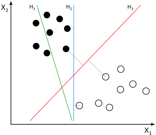
Concept of Hyperplanes and Decision Boundaries in Support Vector Machines:

Hyperplanes:

In the Support Vector Machines (SVMs) context, a hyperplane is a fundamental concept that serves as the decision boundary for classifying data points. In a two-dimensional space, a hyperplane is a line. And in higher dimensions, it becomes a hyperplane. The primary goal of SVM is to find the optimal hyperplane that best separates data points of different classes.

1. Linear Separation:
   • The hyperplane achieves linear separation by creating a boundary that maximizes the margin between the classes. SVM looks for the hyperplane that maximizes the distance to the nearest data points of each class, known as the margin.
2. Mathematical Representation:
   • Mathematically, the equation of the hyperplane is expressed as w⋅x+b=0w⋅x+b=0. Where ww is the weight vector, xx is the input feature vector, and bb is the bias term. The vector ww is perpendicular to the hyperplane and determines the orientation of the decision boundary.
3. Optimal Hyperplane:
   • The optimal hyperplane is the one that maximizes the margin while correctly classifying all training data. It is positioned to have an equal distance from each class’s nearest support vectors (data points closest to the hyperplane).

Decision Boundaries:

1. Margin:
   • The margin is the distance between the hyperplane and the nearest support vectors. Maximizing the margin is crucial for SVM because a larger margin indicates a more robust and generalizable decision boundary.
2. Support Vectors:
   • Support vectors are the data points that lie closest to the hyperplane. They are critical in defining the decision boundary and are the focus of SVM optimization. These support vectors influence the optimal hyperplane.
3. Class Assignment:
   • The decision boundary created by the hyperplane determines the classification of new, unseen data points. If a data point lies on one side of the hyperplane, it is assigned to one class. And if it lies on the other side, it is assigned to the other class. The sign of w⋅x+bw⋅x+b dictates the class assignment.

Non-Linearity and Kernels:

In cases where the data is not linearly separable in the original feature space, SVMs use kernel functions to map the data into higher-dimensional spaces implicitly. This transformation enables the creation of hyperplanes that can effectively separate non-linearly separable data.

Hyperplanes and decision boundaries are central to the functionality of Support Vector Machines. With its associated margin, the optimal hyperplane defines a clear boundary between classes. The concept of support vectors ensures that the decision boundary is robust and generalizes well to new data. The elegance of SVM lies in its ability to create effective linear or non-linear decision boundaries for accurate and reliable classification.

Role of Support Vectors and Margins in Support Vector Machine (SVM) Algorithms:

Support Vectors:

Support vectors are crucial elements in Support Vector Machines’ (SVMs) functioning. They are the data points that lie closest to the decision boundary or hyperplane. The significance of support vectors in SVM lies in their role in defining the optimal hyperplane and influencing the margin. Here is a breakdown of their role:

1. Determining Decision Boundary:
   • Support vectors are the points that have the smallest margin or distance to the decision boundary. They essentially “support” the determination of the optimal hyperplane by influencing its position.
2. Influencing Hyperplane Orientation:
   • The optimal hyperplane is positioned in such a way that it maintains an equal distance from the nearest support vectors of each class. This ensures that the decision boundary is strategically placed to achieve the maximum margin.
3. Robustness to Outliers:
   • Since the position of the hyperplane is heavily influenced by support vectors, SVMs are inherently robust to outliers. Outliers are farther from the decision boundary. They have less impact on the determination of the optimal hyperplane.
4. Reducing Overfitting:
   • Focusing on support vectors contributes to a more generalizable model. By paying attention to the critical data points near the decision boundary, SVM avoids overfitting and ensures that the model can perform well on new, unseen data.

Margins:

The margin in SVM is the distance between the decision boundary (hyperplane) and the nearest data points of each class (support vectors). Maximizing this margin is a central objective in SVM. And it has several implications for the performance and generalization of the model.

1. Robustness to Variability:
   • A larger margin provides a wider separation between classes. That is making the decision boundary more robust to variations in the data. This robustness is crucial for the model’s ability to classify new, unseen instances accurately.
2. Generalization to Unseen Data:
   • Maximizing the margin is synonymous with maximizing the space between classes. A wider margin indicates better generalization to new data points as the model has learned a decision boundary that is less likely to be influenced by noise or outliers.
3. Trade-Off with Misclassification:
   • The margin is optimized while ensuring the correct classification of training data. SVM finds a balance between maximizing the margin and correctly classifying data points. This trade-off contributes to creating an effective and accurate decision boundary.
4. Margin and Hyperplane Relationship:
   • The optimal hyperplane is positioned to have the maximum margin. And the margin itself is a function of the distance between the hyperplane and support vectors. These elements are interconnected in the SVM optimization process.

Support vectors and margins play integral roles in the effectiveness of Support Vector Machines. Support vectors influence the positioning of the decision boundary. It ensures critical data points affect it. Maximizing the margin contributes to the robustness and generalization capabilities of the model. That strikes a balance between precision and flexibility in classification tasks.

Mathematical Aspects of SVM

The mathematical foundation of Support Vector Machines (SVM) involves formulating an optimization problem to find the optimal hyperplane. Here is a step-by-step illustration of the mathematical aspects of SVM:

1. Mathematical Representation of the Hyperplane:

• In a two-dimensional space, the hyperplane equation is given by w⋅x+b=0w⋅x+b=0. Where ww is the weight vector perpendicular to the hyperplane, xx is the input feature vector, and bb is the bias term. The goal is to determine the optimal values for ww and bb.

2. Decision Function:

• The decision function for a new data point xixi is given by f(xi)=w⋅xi+bf(xi)=w⋅xi+b. The sign of this function determines the class to which xixi belongs: f(xi)>0f(xi)>0 for one class and f(xi)<0f(xi)<0 for the other.

3. Margin and Support Vectors:

• The margin is the distance between the hyperplane and the nearest support vectors. Mathematically, the margin MM is given by the reciprocal of the magnitude of the weight vector: M=1∥w∥M=∥w∥1. Maximizing MM is equivalent to minimizing ∥w∥∥w∥, which is the same as minimizing 12∥w∥221∥w∥2 for mathematical convenience.

4. Optimization Problem:

• The optimization problem for SVM is formulated as follows:

Minimize 12∥w∥2 subjects to yi(w⋅xi+b)≥1 for all i,Minimize 21∥w∥2 subject to yi(w⋅xi+b)≥1 for all i,

where yiyi is the class label (+1 or -1) of data point xixi. The constraint yi(w⋅xi+b)≥1yi(w⋅xi+b)≥1 ensures that all data points are correctly classified and lie on the correct side of the decision boundary.

5. Lagrange Multipliers:

• Introduce Lagrange multipliers (αiαi) to handle the inequality constraints. The Lagrangian function (LL) is then defined as:

L(w,b,α)=12∥w∥2−∑i=1Nαi[yi(w⋅xi+b)−1],L(w,b,α)=21∥w∥2−∑i=1Nαi[yi(w⋅xi+b)−1],

Where NN is the number of data points.

6. Derivation and Dual Formulation:

• Minimizing the Lagrangian with respect to ww and bb and substituting the results back into the Lagrangian leads to the dual problem. The dual problem, which involves maximizing the Lagrangian with respect to αα, is expressed as:

Maximize W(α)=∑i=1Nαi−12∑i=1N∑j=1Nαiαjyiyj(xi⋅xj),Maximize W(α)=∑i=1Nαi−21∑i=1N∑j=1Nαiαjyiyj(xi⋅xj),

subject to αi≥0αi≥0 and ∑i=1Nαiyi=0∑i=1Nαiyi=0.

7. Solving the Dual Problem:

• The solution to the dual problem yields the optimal values of αα. From which ww and bb can be determined. The support vectors are the data points corresponding to non-zero αiαi.

8. Decision Boundary:

• The decision function for classifying a new data point xx becomes f(x)=∑i=1Nαiyi(xi⋅x)+bf(x)=∑i=1Nαiyi(xi⋅x)+b, where the sum is over all support vectors.

The mathematical aspects of SVM involve formulating an optimization problem. It introduces Lagrange multipliers and derives the dual problem. Besides, it solves the optimal hyperplane parameters. Optimization ensures that the decision boundary maximizes the margin while correctly classifying the training data.

Types of SVM Kernels

Support Vector Machines (SVMs) are versatile algorithms that can be applied to both linearly and non-linearly separable data. The introduction of kernel functions implicitly allows SVMs to map the input data into a higher-dimensional space. And that is making non-linear relationships discernible in the original feature space. Here are some common types of SVM kernels.

1. Linear Kernel:

• Mathematical Form: K(x,y)=x⋅y+cK(x,y)=x⋅y+c
• The linear kernel is the simplest and is used for linearly separable data. It represents the inner product of the original feature space.

2. Polynomial Kernel:

• Mathematical Form: K(x,y)=(x⋅y+c)dK(x,y)=(x⋅y+c)d
• The polynomial kernel introduces non-linearity by raising the inner product to a power dd. The degree (dd) determines the level of non-linearity.

3. Radial Basis Function (RBF) or Gaussian Kernel:

• Mathematical Form: K(x,y)=e−∥x−y∥22σ2K(x,y)=e−2σ2∥x−y∥2
• The RBF kernel is a popular choice for handling non-linear relationships. It measures the similarity between data points based on the Euclidean distance. The parameter σσ controls the width of the Gaussian.

4. Sigmoid Kernel:

• Mathematical Form: K(x,y)=tanh⁡(αx⋅y+c)K(x,y)=tanh(αx⋅y+c)
• The sigmoid kernel is used for mapping data into a space of hyperbolic tangent functions. It is suitable for data that may not be linearly separable in the original feature space.

5. Laplacian Kernel:

• Mathematical Form: K(x,y)=e−∥x−y∥σK(x,y)=e−σ∥x−y∥
• Similar to the RBF kernel, the Laplacian kernel measures the similarity between data points based on the Euclidean distance. It tends to emphasize sparser regions in the input space.

6. Bessel Function Kernel:

• Mathematical Form: K(x,y)=Jn(β∥x−y∥)K(x,y)=Jn(β∥x−y∥)
• The Bessel Function kernel introduces a Bessel function of the first kind. JnJn denotes it. This kernel is used for certain applications, particularly in image analysis.

7. Custom Kernels:

• SVMs also allow the use of custom kernels tailored to specific applications. These can be designed based on domain knowledge to capture specific relationships in the data.

Choosing a Kernel:

The kernel’s choice depends on the data’s characteristics and the problem at hand. Linear kernels are suitable for linearly separable data. At the same time, non-linear kernels like RBF and polynomial kernels are effective for more complex relationships. The selection of kernel parameters, like the degree in polynomial kernels or the width in RBF kernels, requires careful tuning to achieve optimal performance. Cross-validation is often used to find the best combination of kernel and parameters for a given dataset.

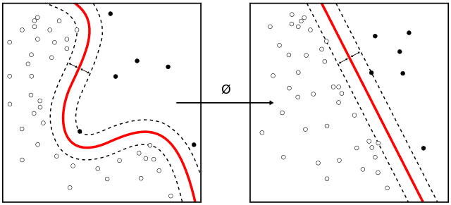
Concept of Kernels in SVM

The concept of kernels in Support Vector Machines (SVM) is a key aspect that enhances the algorithm’s ability to handle non-linearly separable data. Kernels enable SVMs to map input data into a higher-dimensional space implicitly. That makes it possible to find optimal hyperplanes in these transformed spaces. This transformation allows SVMs to tackle complex relationships effectively that may not be discernible in the original feature space. Let us delve into the concept of kernels in SVM:

1. Linearly Inseparable Data:

• SVMs, in their basic form, are well-suited for linearly separable data. In which a straight line (or hyperplane in higher dimensions) can effectively separate different classes. However, real-world data often exhibits more complex, non-linear relationships.

2. Mapping to Higher-Dimensional Space:

• Kernels in SVM solve the non-linearity challenge by implicitly mapping the input data into a higher-dimensional space. This transformation is achieved through the use of a kernel function.

3. Kernel Function:

• A kernel function K(x,y)K(x,y) computes the inner product of the transformed feature vectors ϕ(x)ϕ(x) and ϕ(y)ϕ(y) in the higher-dimensional space without explicitly calculating the transformation itself. Mathematically, K(x,y)=ϕ(x)⋅ϕ(y)K(x,y)=ϕ(x)⋅ϕ(y).

4. Common Kernels:

• Different kernel functions, like linear, polynomial, radial basis function (RBF), sigmoid, and more, are employed based on the nature of the data and the desired transformation.

5. Linear Kernel:

• The linear kernel is the simplest and corresponds to no transformation (ϕ(x)=xϕ(x)=x). It computes the inner product of the original feature vectors.

6. Non-Linear Kernels:

• Polynomial, RBF, sigmoid, and other non-linear kernels introduce various levels of complexity to the transformation. It allows SVM to capture intricate patterns in the data.

7. Kernel Trick:

• The use of kernels is often referred to as the “kernel trick.” It is called a trick because it avoids explicitly computing the transformed feature vectors. That could be computationally expensive for high-dimensional spaces.

8. Support Vector Machines in Transformed Space:

• In the transformed space, SVM seeks an optimal hyperplane that linearly separates the data. The decision boundary in this space corresponds to a non-linear decision boundary in the original feature space.

9. Parameter Tuning:

• The choice of the kernel and its parameters (e.g., the degree in a polynomial kernel or the width in an RBF kernel) requires careful tuning to achieve optimal performance. Cross-validation is often employed to find the best combination for a given dataset.

Kernels in SVMs provide a powerful mechanism to address non-linear relationships in data. It implicitly maps data into higher-dimensional spaces. SVMs can handle complex patterns and capture information that may be hidden in the original feature space. The flexibility of choosing different kernel functions makes SVM a versatile tool for a wide range of applications.

Popular Kernel Functions

1. Linear Kernel:

• Mathematical Form: K(x,y)=x⋅y+cK(x,y)=x⋅y+c
• The linear kernel is the most straightforward. It represents the inner product of the original feature vectors.
• When to Use:
  • Use the linear kernel when the data is approximately linearly separable.
  • It is suitable when there is a clear linear boundary between classes.

2. Polynomial Kernel:

• Mathematical Form: K(x,y)=(x⋅y+c)dK(x,y)=(x⋅y+c)d
• The polynomial kernel introduces non-linearity by raising the inner product to a power dd. The degree (dd) controls the level of non-linearity.
• When to Use:
  • Use the polynomial kernel when the decision boundary is expected to be of a higher degree (curved).
  • Suitable for situations where there are polynomial relationships between features.

3. Radial Basis Function (RBF) or Gaussian Kernel:

• Mathematical Form: K(x,y)=e−∥x−y∥22σ2K(x,y)=e−2σ2∥x−y∥2
• The RBF kernel is a popular choice for handling non-linear relationships. It measures the similarity between data points based on the Euclidean distance. The parameter σσ controls the width of the Gaussian.
• When to Use:
  • Use the RBF kernel when dealing with non-linear and complex relationships.
  • Suitable when there is no prior knowledge about the data distribution.

Choosing Between Kernels:

1. Linear Kernel:
   • Advantages:
     • Simplicity and computational efficiency.
     • Suitable for high-dimensional spaces.
   • When to Choose:
     • When the data is approximately linearly separable.
     • When the dimensionality of the feature space is high.
2. Polynomial Kernel:
   • Advantages:
     • Ability to capture non-linear relationships with higher degrees.
     • Suitable for situations where the decision boundary is expected to be curved.
   • When to Choose:
     • When the data exhibits polynomial relationships.
     • When a higher degree of non-linearity is required.
3. RBF Kernel:
   • Advantages:
     • Versatility in capturing complex non-linear relationships.
     • Effective for a wide range of data distributions.
   • When to Choose:
     • When the data has intricate non-linear patterns.
     • When there is uncertainty about the data distribution.

Considerations for Kernel Selection:

• The choice of kernel depends on the nature of the data and the problem at hand.
• Linear kernels are efficient and suitable for linearly separable data.
• Polynomial and RBF kernels offer flexibility for capturing non-linear relationships. But it may require careful parameter tuning.
• Cross-validation is often used to determine a given dataset’s optimal kernel and associated parameters.

In practice, it’s advisable to experiment with different kernels and parameters to observe their impact on the SVM model’s performance. Then, choose the configuration that best suits a specific problem.

The Impact of Kernel Choice on SVM Performance

The choice of kernel in a Support Vector Machine (SVM) significantly impacts the model’s performance. Different kernels introduce various levels of complexity to the decision boundary. The suitability of a particular kernel depends on the characteristics of the data. Here are critical considerations regarding the impact of kernel choice on SVM performance:

1. Linear Kernel:

• Impact:
  • Well-suited for linearly separable data.
  • Simplicity and computational efficiency.
• When to Use:
  • Choose a linear kernel when the data exhibits a clear linear separation between classes.
  • Suitable for high-dimensional feature spaces.

2. Polynomial Kernel:

• Impact:
  • Introduces non-linearity by raising the inner product to a power.
  • The degree parameter controls the level of non-linearity.
• When to Use:
  • Choose a polynomial kernel when the decision boundary is expected to be of a higher degree (curved).
  • Suitable for situations with polynomial relationships between features.

3. Radial Basis Function (RBF) or Gaussian Kernel:

• Impact:
  • Captures complex non-linear relationships and patterns.
  • The width parameter (σσ) controls the smoothness of the decision boundary.
• When to Use:
  • Choose an RBF kernel when dealing with highly non-linear and intricate relationships.
  • Suitable when there is no prior knowledge about the data distribution.

Considerations:

1. Data Characteristics:
   • The nature of the data plays a crucial role. Linear kernels are effective for linearly separable data. Meanwhile, non-linear kernels like RBF and polynomial kernels are better suited for complex relationships.
2. Overfitting:
   • More complex kernels, like high-degree polynomial or RBF kernels with a small bandwidth, may lead to Overfitting. It is essential to strike a balance between capturing complex patterns. Further, it needs to avoid overfitting to training noise.
3. Computational Complexity:
   • Linear kernels are computationally efficient. That makes them suitable for large datasets or high-dimensional feature spaces. More complex kernels may increase training time and resource requirements.
4. Parameter Tuning:
   • Kernels often have associated parameters (degree in polynomial kernels, σσ in RBF kernels). Proper tuning of these parameters is crucial for optimal performance. Grid search or other optimization techniques can be employed to find the best combination.
5. Cross-Validation:
   • Cross-validation is a valuable tool for evaluating the performance of different kernels on a given dataset. It helps prevent overfitting to the training data and ensures that the chosen kernel generalizes well to new, unseen data.
6. Domain Knowledge:
   • Consider any domain-specific knowledge about the data distribution. Prior knowledge about the problem can sometimes guide the choice of a suitable kernel.

The impact of kernel choice on SVM performance is substantial and should be carefully considered. It involves a trade-off between capturing the complexity of the underlying data patterns and avoiding Overfitting. Experimentation with different kernels and parameters, coupled with thorough cross-validation, is primary to selecting the optimal configuration for a specific problem.

Advantages of Support Vector Machine (SVM) Algorithms

Support Vector Machines (SVMs) offer several advantages, making them a popular and powerful tool in machine learning. Here are some key advantages of SVM:

1. Effective in High-Dimensional Spaces:

• SVMs perform well in high-dimensional feature spaces. That makes them suitable for scenarios where the number of features is significant. This is crucial in modern datasets where numerous variables often represent information.

2. Robust to Overfitting:

• SVMs are less prone to Overfitting. That is especially true in high-dimensional spaces. SVMs create decision boundaries that generalize well to new, unseen data by focusing on the critical support vectors near the decision boundary.

3. Versatility with Kernels:

• SVMs can handle both linearly and non-linearly separable data through the use of kernel functions. These functions implicitly map data into higher-dimensional spaces. That is making complex relationships discernible and expanding the applicability of SVMs to a wide range of problems.

4. Effective in Cases of Limited Data:

• SVMs are effective even when the number of samples is less than the number of features. They are particularly useful in scenarios where data is scarce.

5. Robustness to Outliers:

• The choice of the optimal hyperplane in SVM is influenced by support vectors—data points that are closest to the decision boundary. This approach makes SVM robust to outliers, as the impact of outliers is mitigated by focusing on the critical support vectors.

6. Global Optimization:

• SVM training involves solving a convex optimization problem. It ensures that the algorithm converges to the global minimum. This contrasts with other machine learning algorithms that may converge to local minima.

7. Clear Geometric Interpretation:

• SVMs provide a clear geometric interpretation. The optimal hyperplane is the one that maximizes the margin between different classes. Support vectors define the decision boundary. This geometric interpretation makes SVMs intuitive to understand.

8. Applicability Across Domains:

• SVMs find applications in diverse fields. That includes image and speech recognition, text categorization, bioinformatics, finance, and more. Their versatility and effectiveness make them a popular choice in various real-world scenarios.

9. Memory Efficiency:

• Once the SVM model is trained, only a subset of training points (support vectors) is needed for prediction. This makes SVMs memory-efficient. That is especially true in scenarios with large datasets.

10. Works Well with Small and Medium-Sized Datasets:

• SVMs are well-suited for datasets of small to medium size. They can provide reliable results even when the number of instances is not very large.

Support Vector Machines have demonstrated success in a variety of applications. Their robustness, versatility, and ability to handle complex relationships make them a valuable tool in the machine learning toolkit.

Strengths of SVM Algorithms

Support Vector Machines (SVMs) exhibit several strengths that contribute to their effectiveness in various machine learning applications. Here are some primary strengths of SVM algorithms:

1. Effective in High-Dimensional Spaces:

• Strength:
  • SVMs perform well in high-dimensional feature spaces.
• Explanation:
  • In scenarios where the number of features is significant, like in image and text data, SVMs maintain their effectiveness. The ability to handle high-dimensional data is crucial in modern datasets.

2. Versatility with Kernels:

• Strength:
  • SVMs can handle both linearly and non-linearly separable data through the use of kernel functions.
• Explanation:
  • It introduces non-linearity through kernels like polynomial or radial basis function (RBF). SVMs can capture complex relationships in the data. This versatility expands the applicability of SVMs to a wide range of problems.

3. Robust to Overfitting:

• Strength:
  • SVMs are less prone to Overfitting.
• Explanation:
  • SVMs focus on critical support vectors near the decision boundary. That leads to decision boundaries that generalize well to new, unseen data. This robustness to Overfitting is especially valuable in scenarios with limited data.

4. Robustness to Outliers:

• Strength:
  • SVMs are robust to outliers.
• Explanation:
  • Support vectors influence the determination of the optimal hyperplane—data points closest to the decision boundary. Outliers, being farther from the decision boundary, have less impact on the positioning of the hyperplane. That is making SVMs robust to noisy data.

5. Clear Geometric Interpretation:

• Strength:
  • SVMs provide a clear geometric interpretation.
• Explanation:
  • The optimal hyperplane maximizes the margin between different classes. Support vectors define the decision boundary. This geometric interpretation makes SVMs intuitively understandable and facilitates better insight into the model’s behavior.

6. Global Optimization:

• Strength:
  • SVM training involves solving a convex optimization problem. That is ensuring convergence to the global minimum.
• Explanation:
  • Unlike some other machine learning algorithms that may converge to local minima. SVMs guarantee a global minimum during the optimization process. That is leading to a more reliable model.

7. Applicability Across Domains:

• Strength:
  • SVMs find applications in diverse fields.
• Explanation:
  • Due to their effectiveness and versatility, SVMs are widely applied in image and speech recognition, text categorization, bioinformatics, finance, and other domains. This broad applicability showcases their adaptability to various real-world scenarios.

8. Memory Efficiency:

• Strength:
  • Once trained, SVM models only require a subset of training points (support vectors) for prediction.
• Explanation:
  • This memory efficiency is particularly advantageous in scenarios with large datasets. It needs only the crucial support vectors to be stored for making predictions.

Combining these strengths makes SVMs a powerful and widely used tool in machine learning. That is especially true in scenarios where data exhibits complex relationships, high dimensionality, or limited samples.

Robustness of SVM in Dealing with Overfitting

Support Vector Machines (SVMs) are known for their robustness in dealing with Overfitting. That is especially true when compared to some other machine learning algorithms. Here are several aspects that contribute to the robustness of SVMs in handling Overfitting:

1. Focus on Support Vectors:

• SVMs focus on critical support vectors, which are the data points closest to the decision boundary. These support vectors play a significant role in determining the optimal hyperplane. By concentrating on these crucial data points, SVMs inherently filter out noise and outliers that may lead to Overfitting.

2. Maximization of Margin:

• SVMs aim to maximize the margin between different classes. Margin is the distance between the decision boundary (hyperplane) and the nearest support vectors. A larger margin provides a more robust decision boundary that generalizes well to new, unseen data. This emphasis on maximizing the margin helps SVMs resist Overfitting.

3. Regularization Parameter (C):

• The regularization parameter CC in SVMs controls the trade-off between achieving a low training error and a large margin. A smaller CC encourages a larger margin but may allow some training errors. That is contributing to better generalization. By adjusting the regularization parameter, practitioners can influence the model’s behavior and mitigate Overfitting.

4. Global Optimization:

• SVM training involves solving a convex optimization problem. Optimization ensures convergence to the global minimum. Unlike algorithms that may be sensitive to the initialization and convergence to local minima, SVM’s convex optimization contributes to a more stable and globally optimal solution.

5. Kernel Trick and Non-Linearity:

• The ability to use kernel functions allows SVMs to handle non-linear relationships. While non-linear kernels can introduce complexity, choosing an appropriate kernel and its parameters will enable practitioners to control the degree of non-linearity and avoid Overfitting.

6. Cross-Validation:

• Cross-validation is a common practice in SVM model selection. Practitioners can assess the model’s performance on unseen data by partitioning the dataset into training and validation sets. Cross-validation helps identify an optimal configuration. That includes the choice of kernel and associated parameters. And that generalizes well to new instances.

7. Sparse Model Representation:

• Once the SVM model is trained, only a subset of training points (support vectors) is needed for prediction. This sparse representation contributes to memory efficiency and helps avoid overfitting the training data.

8. Careful Tuning of Hyperparameters:

• Proper tuning of hyperparameters, including the choice of kernel, kernel parameters, and the regularization parameter CC, is crucial to balancing fitting the training data well and generalizing it to new data. This careful tuning is essential for controlling Overfitting.

The focus on support vectors emphasizes margin maximization. The role of the regularization parameter and the ability to handle non-linear relationships through kernels contribute to the robustness of SVMs in dealing with Overfitting. However, it’s important to note that effective use of SVMs requires thoughtful consideration and tuning of hyperparameters based on the characteristics of the data.

Limitations and Challenges

While Support Vector Machines (SVMs) offer several advantages, they also have limitations and challenges that should be considered when applying them to various machine learning tasks. Here are some notable limitations and challenges associated with SVMs.

1. Sensitivity to Noise and Outliers:

• SVMs can be sensitive to noise and outliers. That is especially true when using non-linear kernels. Outliers that fall near the decision boundary or support vectors can significantly impact the position and orientation of the decision boundary. That is affecting the model’s performance.

2. Computational Complexity:

• Training an SVM can be computationally expensive. That is particularly true when dealing with large datasets. The time complexity of SVM training is generally between O(n2)O(n2) and O(n3)O(n3). In which nn is the number of training instances. This can be a limitation in scenarios where training time is a critical factor.

3. Memory Usage:

• SVMs can become memory-intensive, especially when dealing with a large number of support vectors or high-dimensional feature spaces. The need to store support vectors for prediction can impact memory usage. That is making SVMs less suitable for resource-constrained environments.

4. Difficulty in Interpreting the Model:

• SVMs provide a clear geometric interpretation. And the resulting models can be challenging to interpret. That is especially true in high-dimensional spaces. Understanding the significance of individual features or explaining the decision boundary can be complex.

5. Limited Handling of Missing Data:

• SVMs do not handle missing data well. It is essential to preprocess data to handle missing values before applying SVMs, as the algorithm is not inherently designed to handle feature-wise missing data.

6. Parameter Sensitivity:

• SVM performance is influenced by the choice of hyperparameters, like the regularization parameter CC and kernel parameters. Tuning these parameters correctly is crucial. And the performance of the model can be sensitive to their values.

7. Limited Scalability:

• SVMs may face challenges in scalability, especially in large-scale and distributed computing environments. Training large datasets with traditional SVM implementations can be resource-intensive.

8. Handling Imbalanced Datasets:

• SVMs may struggle with imbalanced datasets, where one class has significantly fewer instances than the other. The model may be biased toward the majority class. Therefore, additional techniques may be necessary, like class weighting or resampling.

9. Difficulty in Online Learning:

• SVMs are not well-suited for online learning scenarios. Therefore, the model must be continuously updated as new data becomes available. Re-training an SVM with new data may be computationally expensive.

10. Choice of Kernel Function:

– Selecting the appropriate kernel function and tuning its parameters can be challenging. These choices influence the performance of the SVM model. And improper selection may lead to suboptimal results.

11. Loss of Interpretability in High Dimensions:

– In high-dimensional spaces, especially when using complex non-linear kernels, the interpretability of the model can be lost. Understanding the decision boundaries and the contribution of individual features becomes more challenging.

12. Binary Classification Limitation:

– SVMs are initially designed for binary classification. There are extensions for multi-class classification. The multi-class classification often involves combining multiple binary classifiers. The choice of the strategy may impact performance.

It is essential to consider these limitations and challenges carefully when using SVMs for a particular machine learning task. Additionally, advancements in SVM variants and techniques continue to address some of these challenges. That can improve the overall applicability of SVMs in different scenarios.

Limitations and Challenges Associated with SVM

Support Vector Machines (SVMs) have several limitations and challenges. Their sensitivity to the choice of parameters is a significant concern. Here is a detailed discussion of how parameter sensitivity can impact SVM performance and other associated limitations:

1. Parameter Sensitivity:

• Challenge:
  • SVM performance is highly sensitive to the choice of hyperparameters. That is particularly the regularization parameter CC and kernel parameters.
• Impact:
  • The SVM model may overfit or underfit the data if not carefully tuned. And that may lead to suboptimal performance.

2. Regularization Parameter CC:

• Challenge:
  • The regularization parameter CC controls the trade-off between achieving a low training error and a large margin. The choice of CC influences the model’s bias-variance trade-off.
• Impact:
  • A small CC encourages a larger margin but may allow some training errors. A large CC aims to classify all training points correctly. Potentially, that may lead to Overfitting.

3. Kernel Parameters:

• Challenge:
  • The choice of kernel function and its associated parameters, like the degree in polynomial kernels or the width in RBF kernels, can significantly affect model performance.
• Impact:
  • Inappropriate kernel or parameter choices may result in a model that fails to capture the underlying patterns in the data. And that may lead to poor generalization.

4. Grid Search Complexity:

• Challenge:
  • Exhaustive grid search for the optimal combination of hyperparameters can be computationally expensive, especially in high-dimensional spaces.
• Impact:
  • Time-consuming parameter tuning may hinder the practicality of SVMs in scenarios where computational resources are limited.

5. Handling Imbalanced Datasets:

• Challenge:
  • SVMs may struggle with imbalanced datasets, where one class has significantly fewer instances than the other. The choice of CC may disproportionately influence the model’s behavior.
• Impact:
  • The model may be biased toward the majority class, and additional techniques, such as class weighting, may be required to address the imbalance.

6. Difficulty in Interpretability:

• Challenge:
  • While SVMs provide a clear geometric interpretation, the models can be challenging to interpret, especially in high-dimensional spaces.
• Impact:
  • Understanding the significance of individual features and explaining the decision boundary becomes more complex. That is limiting the interpretability of the model.

7. Memory and Computational Complexity:

• Challenge:
  • SVM training can be computationally expensive, especially with large datasets. The memory requirements for storing support vectors can also be significant.
• Impact:
  • Training time and memory usage may limit the scalability of SVMs in resource-constrained environments.

8. Difficulty in Online Learning:

• Challenge:
  • SVMs are not well-suited for online learning scenarios, where the model needs to be continuously updated with new data.
• Impact:
  • Re-training an SVM with new data may be computationally expensive. And the model may not adapt well to evolving data distributions.

Mitigating Strategies:

1. Cross-Validation:
   • Employ cross-validation to assess the performance of different parameter configurations and select the optimal set.
2. Grid Search with Heuristics:
   • Use grid search with heuristics to explore parameter space efficiently. That is narrowing down potential candidates before fine-tuning.
3. Automated Hyperparameter Tuning:
   • Explore automated techniques, like Bayesian optimization or random search, to streamline the hyperparameter tuning process.
4. Ensemble Methods:
   • Consider using ensemble methods to mitigate the impact of parameter sensitivity by combining multiple SVM models with diverse parameter settings.
5. Feature Scaling:
   • Ensure proper feature scaling, especially when using non-linear kernels. That will help you to avoid undue influence of features with different scales.
6. Model Selection Techniques:
   • Explore model selection techniques, like nested cross-validation, to obtain a more reliable estimate of model performance.

Despite these challenges, SVMs remain a powerful tool. And advancements, like kernel approximations and variations like Support Vector Machines for Support Vector Output (SVMO). Aim to address some of the limitations associated with traditional SVMs. Careful parameter tuning and consideration of these challenges are essential for effectively using SVMs in machine-learning applications.

Scenarios Where SVM Might Not Be the Best Choice

While Support Vector Machines (SVMs) are powerful and versatile, there are scenarios where they might not be the best choice or may face challenges. Here are some situations where alternative machine learning approaches might be more suitable:

1. Large Datasets:

• Challenge:
  • SVMs can be computationally expensive and have a time complexity between O(n2)O(n2) and O(n3)O(n3). That is making them less practical for very large datasets.
• Alternative:
  • For large datasets, algorithms with lower time complexity might be more efficient, like stochastic gradient descent-based methods or tree-based models (e.g., Random Forests, Gradient Boosting).

2. Interpretability Requirements:

• Challenge:
  • SVMs can be challenging to interpret, especially with non-linear kernels or in high-dimensional spaces.
• Alternative:
  • Decision trees or linear models may be preferred when interpretability is a critical requirement since they provide more straightforward explanations for predictions.

3. Imbalanced Datasets:

• Challenge:
  • SVMs may struggle with imbalanced datasets, where one class has significantly fewer instances than the other.
• Alternative:
  • Algorithms with built-in mechanisms to handle class imbalance, like ensemble methods (e.g., Random Forests with class weights) or specialized algorithms (e.g., AdaBoost), might be more appropriate.

4. Online Learning:

• Challenge:
  • SVMs are not well-suited for online learning scenarios where the model needs to be continuously updated with new data.
• Alternative:
  • Incremental learning methods or algorithms designed for online learning, like online gradient descent or mini-batch approaches, are more suitable.

5. Memory Constraints:

• Challenge:
  • SVMs can become memory-intensive, especially when dealing with a large number of support vectors or high-dimensional feature spaces.
• Alternative:
  • Linear models or algorithms with low memory requirements, like logistic regression or linear SVMs, may be more appropriate in memory-constrained environments.

6. Non-Linear Relationships with Limited Resources:

• Challenge:
  • Choosing appropriate kernel and parameter tuning can be challenging when dealing with non-linear relationships and limited computational resources.
• Alternative:
  • Tree-based models like Random Forests or Gradient Boosting effectively capture non-linear relationships and may require less fine-tuning.

7. Noise and Outliers:

• Challenge:
  • SVMs can be sensitive to noise and outliers, and the choice of the kernel may influence this sensitivity.
• Alternative:
  • Robust models or models with built-in outlier detection mechanisms, like robust regression or ensemble methods, may be more suitable.

8. Multi-Class Classification with Many Classes:

• Challenge:
  • While SVMs can handle multi-class classification, the extension from binary to multi-class may involve combining multiple binary classifiers.
• Alternative:
  • Algorithms designed specifically for multi-class problems, like multinomial logistic regression or decision trees, might offer more straightforward implementations.

9. High-Dimensional Sparse Data:

• Challenge:
  • In cases of high-dimensional sparse data, the kernel trick may not provide significant advantages. And the curse of dimensionality may impact SVM performance.
• Alternative:
  • Linear models, especially those designed for sparse data, like logistic regression or linear SVMs, may be more efficient.

10. Natural Language Processing (NLP) Tasks:

• Challenge:

SVMs may not be the first choice for specific NLP tasks where deep learning models, such as recurrent neural networks (RNNs) or transformer models, have shown superior performance.

• Alternative:

Deep learning models are often preferred for tasks like sentiment analysis, machine translation, or language modeling in NLP.

11. Ensemble Learning:

• Challenge:

SVMs may not naturally lend themselves to ensemble methods. And building an ensemble of SVMs might be computationally expensive.

• Alternative:

Ensemble methods like Random Forests or Gradient Boosting are well-suited for building robust models from multiple weak learners.

While SVMs are valuable in many scenarios, understanding their limitations and considering alternative approaches based on the data’s characteristics and the task’s specific requirements is crucial for making informed choices in machine learning applications.

Applications of SVM

Support Vector Machines (SVMs) find applications across various domains due to their versatility and effectiveness in handling both linear and non-linear relationships. Here are some common applications of SVM:

1. Image Classification:

• SVMs are widely used in image classification tasks. In which the goal is to categorize images into different classes. They effectively distinguish objects, scenes, or patterns within images.

2. Handwriting Recognition:

• SVMs have been employed in handwriting recognition systems. The task involves classifying handwritten characters or words. SVMs can effectively handle the non-linear patterns present in different handwriting styles.

3. Face Detection:

• SVMs play a role in face-detection applications. It identifies and classifies faces within images or video frames. SVMs can be trained to distinguish between faces and non-faces. It is contributing much to facial recognition systems.

4. Speech Recognition:

• SVMs are used in speech recognition systems to classify spoken words or phrases. They can handle the complex patterns in audio data and provide accurate classification.

5. Bioinformatics:

• SVMs find applications in bioinformatics. That is particularly true in protein structure prediction, gene classification, and disease diagnosis tasks. They are effective in analyzing biological data with complex patterns.

6. Medical Diagnosis:

• SVMs are utilized in medical diagnosis tasks. That includes the classification of diseases based on patient data, the identification of cancerous cells, and the prediction of medical outcomes.

7. Text and Document Classification:

• SVMs are commonly used in natural language processing tasks, like text and document classification. They can classify documents into categories. That makes them valuable in spam filtering, sentiment analysis, and topic categorization.

8. Financial Forecasting:

• SVMs are employed in financial applications for stock price prediction, credit scoring, and fraud detection. They can capture complex relationships in financial data. And they make predictions based on historical patterns.

9. Quality Control in Manufacturing:

• SVMs are utilized in quality control processes in manufacturing to classify defective and non-defective products based on various features. They help in maintaining product quality and reducing defects.

10. Remote Sensing:

• In remote sensing applications, SVMs are used for land cover classification, vegetation analysis, and identifying objects in satellite imagery. They can handle the multi-dimensional nature of remote sensing data.

11. Gesture Recognition:

• SVMs are applied in gesture recognition systems. They interpret and classify gestures made by users. This is useful in human-computer interaction and device control.

12. Anomaly Detection:

• SVMs can be employed for anomaly detection in various domains, identifying unusual patterns or outliers in data that may indicate errors, fraud, or other irregularities.

13. Network Intrusion Detection:

• SVMs are used for detecting network intrusions by analyzing network traffic patterns. They can classify normal and anomalous activities. Thereby, they are helping to enhance cybersecurity.

14. Environmental Modeling:

• SVMs find applications in environmental modeling, such as predicting air quality, water quality, and climate patterns. They can analyze complex environmental data and make predictions or classifications.

15. Human Activity Recognition:

• SVMs are applied in recognizing human activities from sensor data, such as accelerometers or gyroscopes in Smartphones or Wearables. They can classify activities like walking, running, or sitting.

These applications demonstrate the wide range of domains where SVMs can be effectively applied. And they can showcase their adaptability to diverse data types and problem scenarios.

Examples of Real-World Applications

Support Vector Machines (SVMs) have been successfully applied in various real-world applications across different domains. Here are examples of such applications:

1. Image Classification:

• Example: SVMs are used for classifying images in medical imaging, like identifying cancerous and non-cancerous tissues in mammograms or distinguishing between different types of cells in pathology slides.

2. Text Categorization and Spam Filtering:

• Example: SVMs are employed in email filtering systems to categorize emails as spam or non-spam. They analyze the content and patterns in emails to make accurate classification decisions.

3. Handwritten Character Recognition:

• For example: SVMs have been utilized to recognize handwritten characters. That makes them valuable in applications like check reading in banking or digitizing historical documents.

4. Speech Recognition:

• Example: SVMs are applied in speech recognition systems. They help classify spoken words or phrases. This is useful in voice-activated systems and virtual assistants.

5. Bioinformatics:

• Example: SVMs are employed in bioinformatics to predict protein structure. They can classify genes based on expression patterns and identify potential drug candidates.

6. Financial Forecasting:

• Example: SVMs are used in predicting stock prices and financial market trends. They analyze historical stock data and identify patterns that can inform investment decisions.

7. Face Detection and Recognition:

• Example: SVMs are applied in facial detection and recognition systems. They assist in tasks like unlocking Smartphones using facial recognition or identifying individuals in security applications.

8. Medical Diagnosis:

• Example: SVMs are utilized in medical diagnosis, including the classification of diseases based on patient data. For instance, they may assist in diagnosing conditions like diabetes or neurological disorders.

9. Quality Control in Manufacturing:

• Example: SVMs are used in manufacturing for quality control, helping classify products as defective or non-defective based on features such as size, shape, or color.

10. Remote Sensing:

• Example: SVMs are applied in remote sensing for land cover classification, vegetation analysis, and the identification of objects in satellite imagery.

11. Gesture Recognition:

• Example: SVMs are employed to recognize gestures made by users. They are enabling gesture-based control in applications like gaming or virtual reality.

12. Anomaly Detection in Network Security:

• Example: SVMs are used in network security for anomaly detection. And they are helping identify unusual patterns or behaviors in network traffic that may indicate a security threat.

13. Human Activity Recognition:

• Example: SVMs are applied to recognize human activities from sensor data in Smartphones or Wearables. They can classify activities like walking, running, or sitting.

14. Drug Discovery:

• Example: SVMs are utilized in drug discovery processes to predict the biological activity of molecules. They assist in identifying potential drug candidates.

15. Environmental Modeling:

• Example: SVMs are applied in environmental modeling for predicting air quality, water quality, and climate patterns based on various environmental variables.

These examples illustrate the versatility of SVMs and their successful application in solving complex problems across different industries and domains. The ability of SVMs to handle both linear and non-linear relationships makes them a valuable tool in various real-world scenarios.

Tips for Implementing SVM

Implementing Support Vector Machines (SVMs) effectively involves careful consideration of various factors. The factors include data preparation, model training, and parameter tuning. Here are some tips for implementing SVMs.

1. Understand Your Data:

• Gain a deep understanding of your data’s characteristics. Consider features, data distribution, and the presence of outliers. SVMs are sensitive to these aspects. Therefore, preprocessing steps like feature scaling and handling outliers may be necessary.

2. Feature Scaling:

• Perform feature scaling to ensure that all features contribute equally to the distance computations. Common scaling methods include standardization (z-score normalization) or scaling to a specific range (min-max scaling).

3. Data Splitting:

• Split your dataset into training and testing sets. This allows you to train your SVM on one subset and evaluate its performance on unseen data. Cross-validation is also useful for tuning hyperparameters and assessing model generalization.

4. Kernel Selection:

• Choose the appropriate kernel function based on the characteristics of your data. Linear kernels are suitable for linearly separable data. At the same time, non-linear kernels like polynomial or radial basis function (RBF) effectively capture complex relationships.

5. Hyperparameter Tuning:

• Perform careful hyperparameter tuning. The choice of parameters, especially the regularization parameter CC and kernel-specific parameters, significantly affects SVM performance. Use techniques like grid search or randomized search to find optimal values.

6. Dealing with Imbalanced Data:

• If your dataset is imbalanced, where one class has significantly fewer instances, consider techniques like class weighting or resampling to address the imbalance. SVMs can be sensitive to class distribution.

7. Kernel Approximations:

• Consider using kernel approximations or linear SVM variants for large datasets or high-dimensional spaces. This can reduce the computational burden while still allowing SVMs to capture complex patterns.

8. Understanding Support Vectors:

• Understand the concept of support vectors. These data points lie closest to the decision boundary and influence the positioning of the hyperplane. Visualizing support vectors can provide insights into the decision boundary.

9. Regularization Parameter CC:

• Experiments with different values of the regularization parameter CC. A smaller CC value encourages a larger margin but may allow some misclassifications. At the same time, a larger CC value aims for correct classifications with a potentially smaller margin.

10. Model Evaluation Metrics:

• Choose appropriate evaluation metrics based on your problem. Metrics like accuracy, precision, recall, F1 score, and the area under the Receiver Operating Characteristic (ROC) curve are commonly used for binary classification.

11. Interpretability Considerations:

• Consider using linear SVMs or kernels that provide more interpretable results if interpretability is crucial. Non-linear kernels may make interpretation more challenging.

12. Handle Outliers:

• SVMs can be sensitive to outliers. Consider preprocessing steps like outlier detection and removal or robust kernel functions to make the model more robust to extreme values.

13. Memory Efficiency:

• Take advantage of the memory efficiency of SVMs. Once the model is trained, only the support vectors are needed for prediction. This is particularly beneficial when dealing with large datasets.

14. Advanced Kernel Tricks:

• Explore advanced kernel tricks, like using custom kernels or combining multiple kernels. These techniques can be beneficial for capturing specific patterns in the data.

15. Ensemble Methods:

• Consider using ensemble methods with SVMs to improve performance. Techniques like bagging or boosting can be applied by combining multiple SVM models to enhance predictive accuracy.

By paying attention to these tips, you can improve the effectiveness and efficiency of your SVM implementation to ensure that it is well-suited to your specific problem and dataset.

Practical Tips for Implementing SVM Algorithms

Here are practical tips for implementing Support Vector Machine (SVM) algorithms.

1. Data Exploration and Preprocessing:

• Tip: Start by exploring and understanding your data. Visualize distributions, handle missing values, and identify outliers. SVMs can be sensitive to these factors.
• Action: Perform data cleaning and normalization and address any data-specific challenges before applying SVM.

2. Feature Scaling:

• Tip: Scale your features. SVMs are distance-based algorithms. Scaling ensures that all features contribute equally to the decision boundary.
• Action: Use standardization (z-score normalization) or min-max scaling to bring features to a similar scale.

3. Data Splitting and Cross-Validation:

• Tip: Split your dataset into training and testing sets. Use cross-validation for hyperparameter tuning to ensure robust model evaluation.
• Action: Use techniques like stratified sampling to maintain class distribution integrity during data splitting.

4. Kernel Selection:

• Tip: Choose the appropriate kernel based on your data’s characteristics. Linear kernels work well for linearly separable data, while non-linear kernels like RBF capture complex patterns.
• Action: Experiment with different kernels and assess their impact on model performance.

5. Hyperparameter Tuning:

• Tip: Invest time in hyperparameter tuning. Parameters like CC and kernel-specific parameters significantly affect SVM performance.
• Action: Use a grid or randomized search to find the optimal hyperparameter values. Consider using a validation set for intermediate evaluations.

6. Handling Imbalanced Data:

• Tip: Address class imbalance issues if present. SVMs can be sensitive to imbalanced datasets.
• Action: Explore techniques such as class weighting or resampling to ensure balanced learning.

7. Understanding Kernel Parameters:

• Tip: Understand the role of kernel parameters (gamma in RBF). These parameters control the flexibility of the decision boundary.
• Action: Experiment with different values and observe their impact on model performance. Visualize decision boundaries for better insight.

8. Parallelization and Memory Efficiency:

• Tip: Take advantage of parallelization options in SVM libraries for faster training.
• Action: Configure your SVM implementation to use parallel processing if available. Optimize memory usage, especially for large datasets.

9. Ensemble Methods:

• Tip: Consider using ensemble methods with SVMs for improved performance.
• Action: Explore techniques like bagging or boosting to combine multiple SVM models and enhance overall predictive accuracy.

10. Visualizing Support Vectors:

• Tip: Visualize support vectors for a better understanding of the decision boundary.
• Action: Plot decision boundaries and support vectors to gain insights into the critical data points influencing the model.

11. Regularization Parameter CC:

• Tip: Experiment with different values of the regularization parameter \(C\) to balance between achieving a low training error and a large margin.
• Action: Understand the impact of \(C\) on the model’s bias-variance trade-off and adjust accordingly.

12. Advanced Kernel Tricks:

• Tip: Explore advanced kernel functions and custom kernels for specific data patterns.
• Action: Experiment with custom kernels or combination strategies to capture complex relationships in the data.

13. Interpretability Considerations:

• Tip: Consider interpretability requirements when choosing the kernel and model type.
• Action: Opt for linear SVMs or kernels that provide more transparent results for greater interpretability.

14. Handling Outliers:

• Tip: Be mindful of outliers, as SVMs can be sensitive to them.
• Action: Consider preprocessing steps, such as outlier detection and removal, or explore robust kernel functions to enhance model robustness.

15. Documentation and Code Comments:

• Tip: Maintain clear documentation and comments in your code for better collaboration and future reference.
• Action: Clearly annotate your code to explain choices made during preprocessing, hyperparameter tuning, and any specific implementation details.

By following these practical tips, you can enhance the effectiveness and efficiency of your SVM implementation. That can lead to better model performance and insights.

Considerations for Parameter Tuning and Model Evaluation

Parameter tuning and model evaluations are crucial to building an effective Support Vector Machine (SVM) model. Consider the following considerations for parameter tuning and model evaluation:

Parameter Tuning:

1. Regularization Parameter (CC):

• Consideration: The regularization parameter CC controls the trade-off between a smooth decision boundary and classifying training points correctly.
• Tuning: Use techniques like grid search or randomized search to explore different CC values. Consider a wide range of values. Use both small and large to find the optimal balance.

2. Kernel Parameters:

• Consideration: Different kernels (linear, polynomial, RBF) have associated parameters (degree, gamma) that impact the shape and flexibility of the decision boundary.
• Tuning: Experiment with different kernel functions and their parameters. For example, for the RBF kernel, vary the values of gamma-gamma to find the optimal setting.

3. Class Weights:

• Consideration: In imbalanced datasets, adjusting class weights can mitigate the impact of the majority class on the SVM.
• Tuning: If dealing with imbalanced data, experiment with different class weightings. Some SVM implementations provide options to assign different weights to classes.

4. Kernel Choice:

• Consideration: The choice of kernel depends on the linearity of the data. Linear kernels are suitable for linearly separable data. At the same time, non-linear kernels capture more complex relationships.
• Tuning: Try different kernels based on the nature of your data—experiment with linear, polynomial, and RBF kernels to find the one that best fits your problem.

5. Cross-Validation:

• Consideration: Cross-validation is essential for assessing model generalization. It helps avoid overfitting the training data.
• Tuning: Use techniques like k-fold cross-validation to split the data into multiple folds. Evaluate the model on different folds and average the results for a more robust performance estimate.

Model Evaluation:

1. Selecting Evaluation Metrics:

• Consideration: The choice of evaluation metrics depends on the nature of the problem (binary classification, multi-class, regression).
• Action: For binary classification, consider metrics like accuracy, precision, recall, F1 score, and the area under the ROC curve. For regression, metrics like mean-squared error or R-squared are common.

2. Confusion Matrix Analysis:

• Consideration: A confusion matrix provides detailed insights into model performance, especially in binary and multi-class classification.
• Action: Analyze the confusion matrix to understand true positives, true negatives, false positives, and false negatives. This can help identify specific areas of model misclassification.

3. ROC Curve and AUC:

• Consideration: The Receiver Operating Characteristic (ROC) curve and area Under the Curve (AUC) are useful for assessing binary classification models, especially in imbalanced datasets.
• Action: Plot the ROC curve and calculate AUC to evaluate the trade-off between sensitivity and specificity.

4. Precision-Recall Curve:

• Consideration: In imbalanced datasets, precision-recall curves provide insights into the trade-off between precision and recall.
• Action: Plot the precision-recall curve and calculate the area under the curve. It’s particularly useful when positive instances are rare.

5. F1 Score:

• Consideration: The F1 score is a harmonic mean of precision and recall. It provides a balanced measure.
• Action: Use the F1 score, especially when there is an uneven class distribution or when both precision and recall are crucial.

6. Bias-Variance Trade-Off:

• Consideration: Evaluate the model’s bias-variance trade-off to understand its generalization performance.
• Action: Analyze how the model performs on the training set versus the validation or test set. If there is a significant gap, the model might be overfitting.

7. Overfitting and Underfitting:

• Consideration: Assess whether the model overfits or underfits the data.
• Action: Monitor training and validation/test performance. If the model performs well on the training set but poorly on unseen data, it may need to be more balanced.

8. Interpretability:

• Consideration: Consider the interpretability of the model, especially in applications where model explanations are crucial.
• Action: Linear SVMs or kernels with more interpretable results may be preferred in scenarios where understanding the decision boundary is essential.

9. Runtime Considerations:

• Consideration: Evaluate the runtime performance, especially for large datasets.
• Action: Measure the training and prediction times. If the computational cost is a concern, explore methods like kernel approximation or linear SVM variants.

10. Ensemble Methods:

• Consideration: If applicable, consider using ensemble methods with SVMs for improved robustness and predictive accuracy.
• Action: Experiment with techniques like bagging or boosting to combine multiple SVM models and enhance overall model performance.

You can build a robust and effective machine learning solution tailored to your specific problem and dataset by carefully tuning parameters and evaluating your SVM model thoroughly. Regularly reassess and refine your model based on ongoing evaluations and any changes in the data distribution.

Conclusion

In conclusion, Support Vector Machines (SVMs) are powerful and versatile machine learning algorithms with a wide range of applications. They excel in both linear and non-linear classification tasks. That makes them valuable tools in various domains like image classification, text categorization, and bioinformatics. Understanding the key concepts of SVMs, including hyperparameters, kernels, and the optimization problem, is crucial for successful implementation.

When working with SVMs, thoughtful consideration of data preprocessing, feature scaling, and parameter tuning significantly impacts model performance. Choosing the correct kernel function and tuning hyperparameters, like the regularization parameter CC and kernel-specific parameters, is essential for achieving optimal results.

Model evaluation is equally important, and careful selection of appropriate metrics based on the problem type ensures a thorough understanding of the model’s performance. Techniques like cross-validation, ROC curves, precision-recall curves, and confusion matrix analysis provide insights into different aspects of model behavior.

While SVMs have proven effective in many scenarios, it’s essential to acknowledge their limitations, like sensitivity to parameters and computational complexity. Awareness of these limitations and considering alternative approaches is crucial for making informed decisions in real-world applications.

As machine learning evolves, SVMs remain a valuable part of the toolkit. Ongoing research and advancements aim to address some of their challenges. By staying informed, implementing best practices, and adapting to the specific requirements of each problem, practitioners can harness the full potential of SVMs for diverse and complex tasks.

Additional Resources

Here are some additional resources to help readers delve deeper into Support Vector Machines (SVMs):

Books:

1. “Support Vector Machines and Other Kernel-Based Learning Methods”
   • Author: Nello Cristianini, John Shawe-Taylor
   • Link: Support Vector Machines and Other Kernel-Based Learning Methods
2. “Hands-On Machine Learning with Scikit-Learn, Keras, and TensorFlow”
   • Author: Aurélien Géron
   • Link: Hands-On Machine Learning with Scikit-Learn, Keras, and TensorFlow

Articles and Tutorials:

1. Scikit-Learn Documentation on SVM:
   • Link: Scikit-Learn SVM Documentation
2. Introduction to Support Vector Machines (SVM) – Towards Data Science:
   • Link: Introduction to Support Vector Machines (SVM)
3. Kernel Methods in Machine Learning – A Gentle Introduction:
   • Link: Kernel Methods in Machine Learning
4. Support Vector Machines (SVM) – Stanford University Lecture Notes:
   • Link: CS229: Machine Learning – SVM

Online Courses:

1. Coursera – “Machine Learning” by Andrew Ng:
   • Link: Machine Learning – Andrew Ng
2. edX – “Support Vector Machines in Machine Learning” by Columbia University:
   • Link: Support Vector Machines in Machine Learning

These resources cover a range of topics from introductory to advanced levels, providing a comprehensive understanding of SVMs and their applications in machine learning. Happy learning!